Introduction
On this page you find a short introduction to the most important parts of how to work with spreadsheets in Microsoft Excel
Cells
In all spreadsheets software, data is kept in a grid. Each box in the grid is called a cell. The grid is divided into columns (identified by by letters) and rows (identified by numbers).
Rows
The rows are numbered. The column number indicates the vertical position of the row. Row 1 is the top row. In the below example, all the cells in row three has been selected.
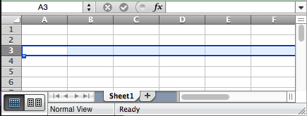
Row 3 in the grid
Columns
The columns are enumerated using letters. The column letter indicates the horizontal position of the column. Column A is the left most column. In the below example, all cells in column C has been selected.
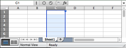
Column C in the grid
Cell references
To refer to a specific cell in the grid, a combination of the column letter(s)
and row number is used. In the below example, C3 refers to the cell in column
C and row 3 in the grid.
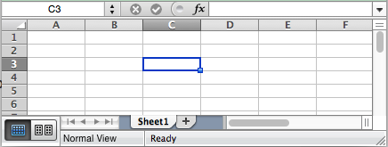
In the grid, cell C3 is located in column C, row 3
Rectangular ranges
A rectangle of connected cells is called a (rectangular) range. A range is
identified by the top left cell and the bottom right cell. The two cell
references used to identify a range are separated by a : (colon).
In the below example, the range A1:C3 has been selected.
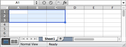
The range A1:C3
Get started
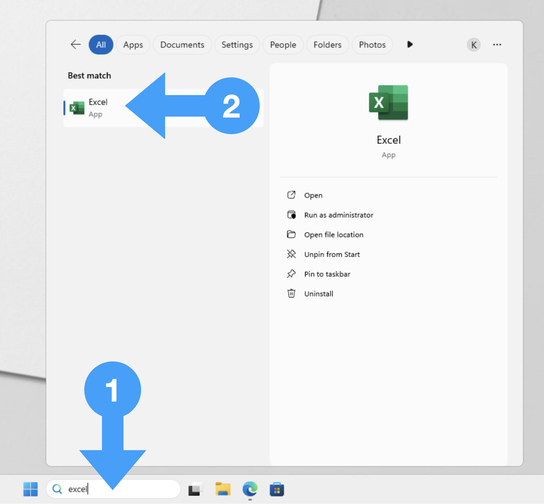
Microsoft excel should be installed on the computers in the computer rooms at the university. To start Excel from a Windows computer in one of the University computer rooms, search for Excel in the taskbar (1) and click on Excel (2).
You may also use your free Microsoft Live account to run excel in your web browser. Note that the online version of Excel does not support trendlines in graphs.
When you start Exel, choose blank page to start a new document. You should now see something similar to this.
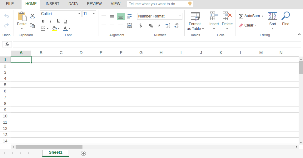
A new Excel document
You can now start entering numbers and text in the cells. Go to the File tab to save the document.
Entering numbers
Excel has many smart functions that helps you entering numbers efficiently. You can test this by typing some numbers (pressing Enter takes you to the next row), highlighting them and clicking and dragging the mouse down from the lower right corner to create a series of numbers based on the selected numbers.
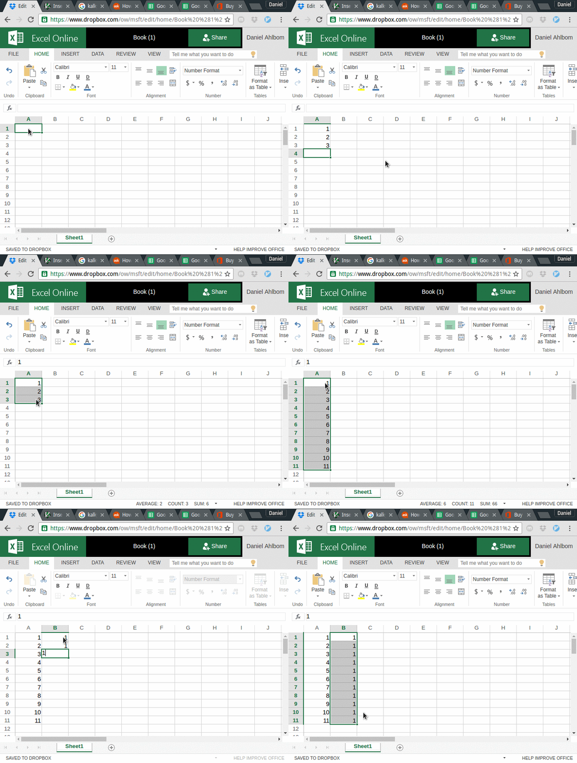
Creating number series
Formulas
In Excel, formulas are a way to perform calculations. You can enter a formula into a cell in two different ways.
Alternative 1:
- Click on the cell where you want to enter a formula.
- Click on \(f_x\) which you will find just above the grid, on the left.
- Type your formula.
Alternative 2:
- Click the cell where you want to enter a formula.
- Type
=followed by the formula you want to enter.
Click on an empty cell and try entering the formula 3 + 5 in the cell. After
pressing enter, the result 8 appears in the cell.
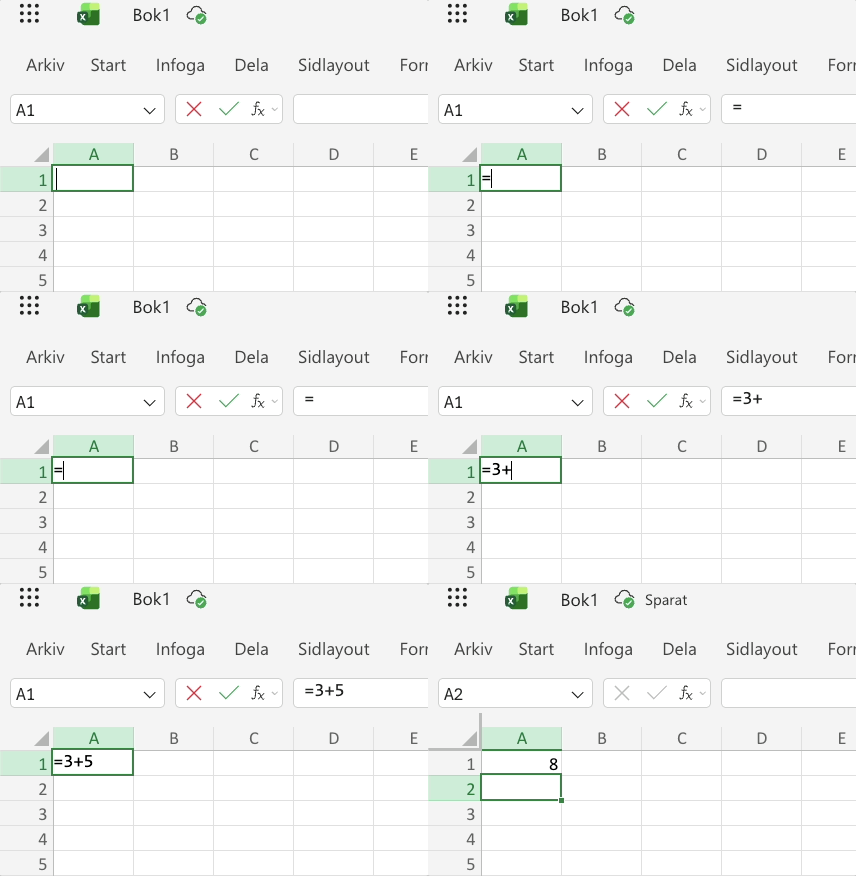
Calculating 3 + 5 using a formula.
Functions
In addition to standard mathematical calculations (+, -, *, /), formulas
can use functions. A function in Excel behaves in the same way as a mathematical
function. A function takes zero or more arguments (input) and calculates a
result (output). Excel has a large number of built-in functions.
By using formulas and functions, you can perform complex calculations in your spreadsheets.
Entering formulas as text
To demonstrate how to manually entering formulas, we use the SUM function. As
the name implies, this function calculates the sum of a number of values.
Before proceeding, make sure you have some values in the range A1:B11.
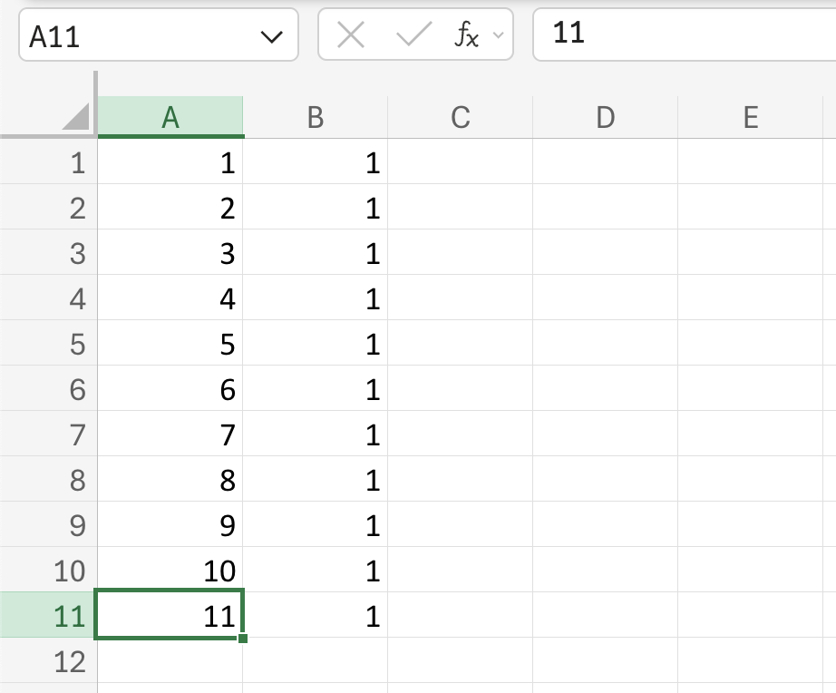
Exempel of values.
In order for Excel to understand that you want to enter a formula in a cell
you must start the formula with = (equal sign), followed by
formula. Arguments to functions must be inside parentheses.
- Click on the cell
A12. - Enter the forumla:
- If you are using Excel in English, type
=SUM(A1:B11). - If you are using Excel in Swedish, type
=SUMMA(A1:B11).
- If you are using Excel in English, type
- Press Enter.
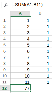
Calculate the sum of all values in the range A1:B11.
In this example, the function name is SUM (English), or SUMMA (Swedish), while the argument is the range A1:B11. After you press Enter, the sum of all numbers in the range A1:B11 is displayed in cell A12. In this example, the sum is 77.
Try changing some values in the range A1:B11 and notice how the sum in cell A12 automatically updates.
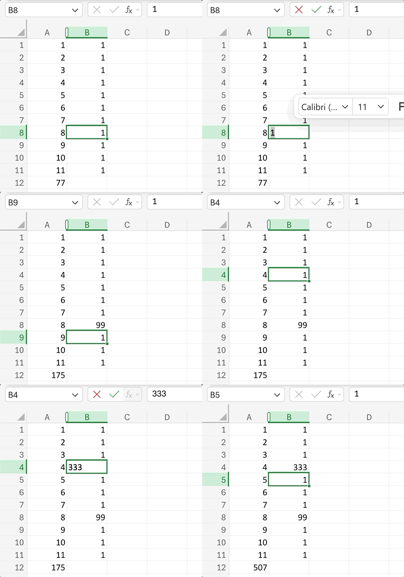
Entering formulas with the mouse.
You can also entering formulas using the mouse.
- Click on a cell.
- Click on Insert -> Function.
- Choose the function you wish to use from the menu.
- Select the range to use as input to the function.
- Finnish the formula by pressing on Enter.
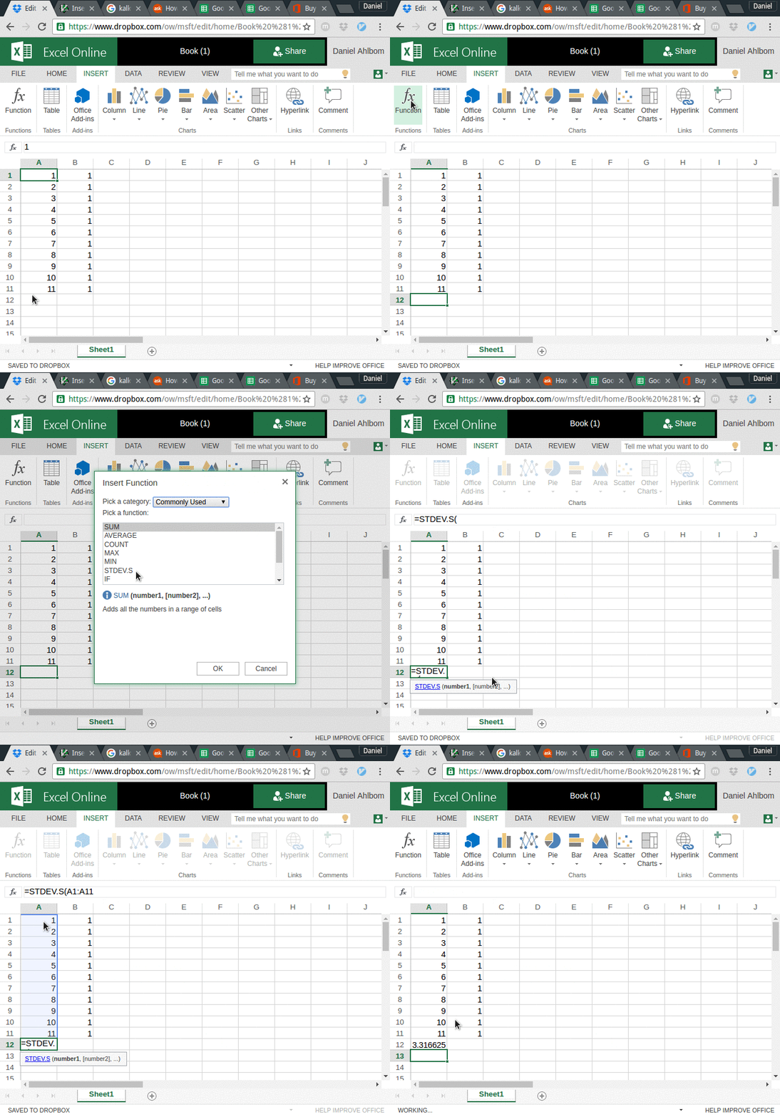
Applying the STDEVS function to the range `A1:A11`
Advanced formulas
You can construct more advanced formulas by combining arithmetic and functions.
- Arithmetic calculation are done using the usual symbols
+(addition),-(subtraction),*(multiplication) and/(division). The symbol^is used for exponentiation. - Parentheses are used for grouping.
- You can combine functions and arithmetic.
- Cell and range references can be us as input to functins.
Let’s look at an example.
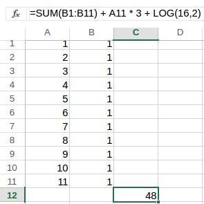
A more advanced formula
In the above example, the formula =SUM(B1:B11) + A11 * 3 + LOG(16,2) has been
entered in the cell C12.
The sum of the range
B1:B11is added to the value in cellA11multiplied by3, finally the2-logof16is added.The formula calculates \(11 + 11 \cdot 3 + 4\) and the result
48is shown in cellC12.
Generate charts
One of the most important features in a spreadsheet is the ability to generate graphical charts. Select the range with data you want to use to create a chart. From the Insert tab, select the kind of chart you want to create.
In the following example, a pie chart is created from the data in the range
A1:B11.
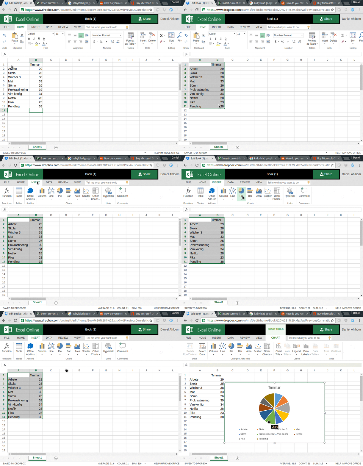
A pie chart of the data in the range `A1:B11`
Editing charts
Once you created a chart the chart the be edited.
Click on the
Chart Titlein the chart to change the title.To edit the chart type and other parameters, double click anywhere on the chart. Now a menu with chart settings will appear.
Trendlines and regression analysis
The goal of regression analysis is to, based on observed data, create a function that describes it. One way to illustrate this is to use trendlines.
- A trendline shows trends in how your data values change (for example, how a metric changes over time).
- The \(R^2\) value (coefficient of
determination) is a measure of the goodness of fit of a model. In regression, the
\(R^2\) coefficient of determination is a statistical measure of how well the
regression predictions approximate the real data points.
- Zero (0.0): No linear fit at all. The trend line explains none of the variation in the data points.
- High value (e.g. above 0.8): Strong relationship and high reliability.
- One (1.0): The regression predictions perfectly fit the data.
- Low value (e.g. below 0.3): Weak relationship; the spread of the data points is large relative to the line
Microsoft Live
The Microsoft Live version of Excel does not support trendlines.
To add a trendline to a chart, first click on the chart. Now the tabs Design, Layout and Format appears to the to upper right (1).
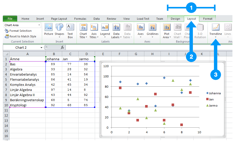
Accessing chart trendline options
From the Layout tab (2), choose Trendline (3) to access the options for adding a trend line to the chart.
You can also click on an already added trendline to access the trendline settings.
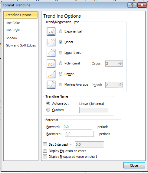
Trendline settings
Graphs are used to present data as clearly as possible. Use colors and other settings to make your graphs as easy as possible to understand.
In the following example, three different data series are represented with different colors and different symbols. Three trendlines with the same colors as the data series have been added.
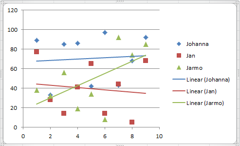
An example showing three different trendlines
In the following example, a trendline has been added to a bar chart.
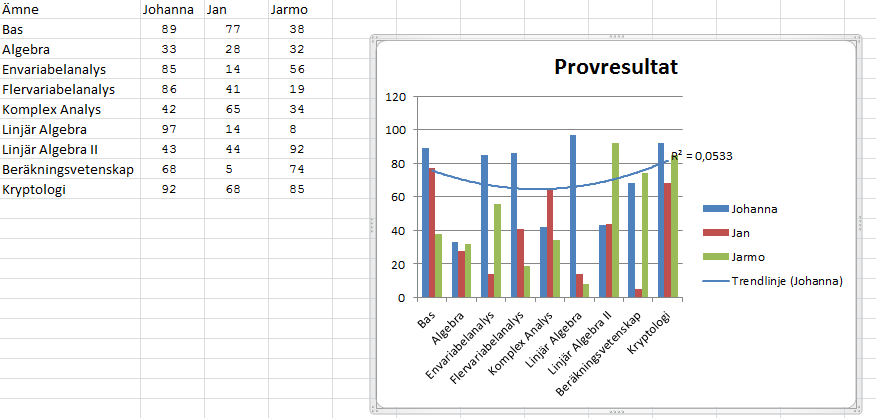
Trendline added to a bar chart
In the above example, random values have been used in the spreadsheet. The
\(R^2\) value for the Johanna trendline is 0.0533, i.e, the trendline is not
a very good fit to the data.